Reversing Factorio's RNG
Published at August 22, 2026
Broken in Factorio 2.1 – Version 2.0 only!
Factorio 2.1 changes the way the RNG is used.
This breaks my in-game implementations. The theoretical aspects of how the RNG works still apply, as they still use the same RNG. For more info see section 6.1. Factorio 2.1.
Introduction
With the release of the Space-Age DLC in Factorio several new mechanics were introduced. One major mechanic was the new concept of different items and building qualities. By default, items are created with common quality. If quality modules are used in the crafting machine we gain a small chance to obtain items of higher quality.
What does that entail? In short: Items and buildings gain improved stats, such as faster crafting speeds, modules providing stronger buffs, power poles having an increased range and inserters swinging faster. Thats pretty neat – hence we are interested in obtaining the highest possible quality on our items and buildings. To source a large number of such items the devs essentially said that this randomness boils down to “basically statistics”,1 i.e. if the volume high quality items one obtains is sufficiently large, then the observed distribution of qualities will be close to the expected distribution.
But is it the only way to scale? Thinking about it, one might ponder:
How is it possible for a deterministic game like Factorio to have a random mechanic?
The short answer is: It isn’t random.
Instead – as is common in computing – the simulation makes use of a pseudo-random number generator (PRNG). A PRNG is a deterministic algorithm which produces a sequence of numbers which for all intents and purposes appears to be random. In particular this means properties like it following a well defined distribution of outputs, which contains no discernable patterns. Normally in computer science one can get away with treating the PRNG as just a black box function which can yield random numbers, without concerning oneself with how it actually works. Yet by taking a look under the hood we can do something funny.
Then we could just run the same algorithm on the state and obtain the same outputs, which will also be seen by the game internally. Its necessarily always the same outputs, as otherwise the chosen algorithm would not be deterministic. As such we can run the same computations simultaneously to the game and predict the future outputs of the PRNG, allowing us to predict the future “random” events which will occur in the game, such as which crafts will observe an increase in quality.
In the following sections I’ll build up to that point, starting from what RNG the game uses, how it is breakable and how it can be abused ingame.
The entire background should be understandable if you have a rudimentary understanding of linear algebra. That should be the only prerequisite.
Starting from Nothing
Soooo, how does one figure out what PRNG algorithm Factorio uses? Afterall, there are several different implementations out there they could have chosen from.
To figure this out, my first step was a rudimentary internet research. As the Factorio community is quite large and filled with many technically inclined individuals, surely someone must have asked this question before. After digging around a bit I found a post on the Factorio forums asking basically the same thing I wanted to know, though 11 years have passed since then. In that thread, we also find the following answer by Cube, a former developer at Wube. They wrote:
[…] We chose taus88 mainly because it is the fastest from boost’s generators. I was thinking of removing one of the three LFSRs (that should make it about 40% (?) faster), but there is no point, since the ran[d]om numbers are not a bottleneck for us.
This already gives us a lead on where to look next: the Boost.Random library.
There we find the following (abbreviated) implementation for the taus88 generator:
typedef xor_combine_engine<
  xor_combine_engine<
    linear_feedback_shift_engine<uint32_t, 32, 31, 13, 12>, 0,
    linear_feedback_shift_engine<uint32_t, 32, 29, 2, 4>, 0>, 0,
  linear_feedback_shift_engine<uint32_t, 32, 28, 3, 17>, 0> taus88;

template<class UIntType, int w, int k, int q, int s>
class linear_feedback_shift_engine {
  // w = word size (e.g. 32 for 32 bit uint)
  // k = number of bits in the LFSR
  // q = feedback tap position
  // s = number of steps to do at once
  // wordmask() = 0b11...111; mask of w low bits set
  result_type operator()() {
    const UIntType b = (((value << q) ^ value) & wordmask()) >> (k-s);
    const UIntType mask = (wordmask() << (w-k)) & wordmask();
    value = ((value & mask) << s) ^ b;
    return value;
  }
}
This means that taus88 consists of 3 linear_feedback_shift_engine whose results are XORed together.
Note that this linear feedback shift engine is more commonly referred to as a linear feedback shift register (LFSR).
Though when starting the project that post was already 8 years old. Hence, I wanted to cross-check the information given on the forum against the most accurate source available: The game binary.
While the game itself is closed source, the developers graciously ship a .pdb file containing the debug symbols alongside the game binary.
This means we can generate a well-annotated decompilation of the binary to inspect the code and figure out what is going on under the hood.
To this end, I used the open source decompilation tool Ghidra, switching to Binary Ninja later on in the project.
Regardless of which tool one uses, one can rather quickly find the RandomGenerator class in the game’s code, where getInt() is implemented as follows:
uint RandomGenerator::getInt(RandomGenerator *this) {
  uint a = this->seed1;
  uint b = this->seed2;
  uint c = this->seed3;

  a = (a << 12 ^ a >> 6) & 0x1fff ^ a >> 19 ^ a << 12;
  b = (b << 4 ^ b >> 23) & 0x7f ^ b >> 25 ^ b << 4;
  c = (c << 17 ^ c >> 8) & 0x1fffff ^ c >> 11 ^ c << 17;

  this->seed1 = a;
  this->seed2 = b;
  this->seed3 = c;

  return a ^ b ^ c;
}
The first thing which stands out is that almost none of the constants used in the original taus88 definition remain.
This can be attributed to the compiler performing optimizations such as constant folding to reduce the number of required operations.
Yet the fact that we store 3 seeds for our RNG state is a first strong indicator that it is indeed the same generator.
Likewise, the states are updated independently of one another, with the final result being the XOR of all three states.
To rid myself of all remaining doubt about whether the two implementations are equivalent, I rewrote both variants in Python so they can be run using sympy, a Python library for symbolic manipulation. Advancing both variants by a single step confirms that all bits of the corresponding registers update in the exact same fashion. I used sympy here because doing these equivalence checks by hand () would have been quite tedious. The corresponding code can be found here.
Ok, with all that established, we are certain that the RNG used in Factorio is indeed the taus88 generator,
which itself is a combination of 3 LFSRs.
This is a very interesting result, as LFSRs are known to be quite weak PRNGs –
in the literature one even finds the statement that they are trivially breakable.2
To understand what makes them ”weak” and how we can exploit this weakness to predict the future RNG calls, we first need to look at the underlying mathematics of LFSRs, which is the subject of the next section.
LFSR Maths Review
To begin, we need to understand what the linear feedback shift register (LFSR) actually models. First, consider a simple register. It describes a collection of bits, aggregated into a single value :
Each individual bit can be seen as a binary variable with . While it is common to consider this register value to represent a number in the range , it is more useful in our case to instead consider the register to actually describe a vector of individual bits, i.e. . Additionally, we consider two operations which operate on each individual bit:
- : The XOR operation takes 2 bits and returns 1 if the bits differ and 0 if they are equal. Note that this is equivalent to addition modulo 2.
- : The AND operation takes 2 bits and returns 1 if both bits are 1, otherwise it returns 0. This is equivalent to multiplication modulo 2.
Now extend that notion of a register into a shift register. To shift, move all bits in the register downwards by taking each higher bit and shifting it 1 position down, dropping the lowest bit as the output. Here we follow the convention that the most significant bit (highest bit) is the leftmost bit and the least significant bit is the rightmost bit .
You can interact with this kind of register below. Tap the individual bits to toggle them, and use the controls to start, stop and step the registers.
Well… This is boring! We converge pretty quickly to the same value of 0 regardless of the initial state. This does not seem random at all! To keep our shift register from always just discarding all information we will add another component, namely some feedback. The first idea is to just loop the discarded lowest bit back into the highest bit, as it previously had no preceding bit from which it could obtain (new) information, while we discard information in the lowest bit. Doing this we have basically implemented a bit roll operation:
Hmmm… At least we no longer always arrive at an empty register. But the sequence when the last bit lights up is very predictable. This is due to the fact that the information that we observe repeats every steps – each bit remains unmodified after all! Thanks to the low cycle length, one can again quickly spot the pattern produced by our current feedback shift register. To combat this we insert some linear feedback, by adding the feedback not only to the first bit, but also some intermediate bits. Note that addition here means XOR, as we are working with individual bits:
Unlike the last steps it might not be immediately obvious why this step is named the way it is. It comes from the fact that the XOR operation we use to combine the feedback into the inner bits causes our bit states to be a linear combination of the previous bit states. This linearity is also the reason why we can reconstruct the internal RNG state from just observations alone, and why standalone LFSRs are cryptographically weak PRNGs.
Note that in all the cases above only the last bit was considered an output. However, in practice it is more common to output the entire register state as the result of the RNG call. This then allows one to reinterpret the number as a proper integer in producing random looking numbers.
We now know how an LFSR gets constructed. In particular, given the state at time we now know how to:
- Generate the next state .
- Generate corresponding output bits, either one at a time, or as a full integer value.
Regarding the Cycle length of LFSRs
The cycle length of an LFSR is the number of steps it takes until the state repeats. For an LFSR with bits, the maximum cycle length is (every state except the all-zero state).
LFSR mechanics are actually also modeled by polynomials over . A single step then corresponds to multiplying the current state with (this shifts the bits up one index).
Finally, by doing this modulo a feedback polynomial of degree that is primitive (and therefore irreducible), we can ensure that the cycle length is maximal, i.e. . then specifies to the spaces where the feedback is inserted, i.e. the bits which are XORed with the feedback bit. In other words, not all feedback configurations are equally good, and the choice of feedback taps is crucial to ensure a long cycle length.
LFSRs are linear
Let us take another look at the linearity claim from above. To do that rather than considering arbitrary instantiations of , i.e. states where all bits were set to either 0 or 1, we can now consider a symbolic representation of the LFSR. We still start at an arbitrary point in time , at which we label each individual bit with an additional symbolic variable . Then we track how the bits evolve over time as we apply the LFSR transition rules. Each symbol is colored either on or off depending on the state at which the LFSR was started. As before, you can toggle individual bits by clicking on them – though only while the bit labels are in the initial state.
We see that every bit is always just a combination of the initial bit states. Note that whenever we observe the cancels out, allowing us to remove it from the equation again. While stepping, each instantiated bit will always stay equal to the parity of “on” bits in the symbolic combination depending on the state when we assigned the labels. Additionally we notice that a bit is either just the preceding bit state, or it is a combination of the preceding and the feedback state.
Now what has this got to do with linearity?
First of all, note that the set of bits joined with the operations and form a structure known as a field. This field is commonly known as the Galois field or the modular arithmetic mod 2. A field is just a math term for a set of values joined with some operations which satisfy a certain set of properties (see below).
Field properties of
The properties which need to be satisfied to declare a field are as follows:
- Associativity (both and ): and .
- Commutativity (both and ): and .
- Identity: For this is : and for this is : .
- Additive Inverse: For any we have a such that . Note that here we have .
- Multiplicative Inverse: For any we have such that is trivial as the only other element is 1.
- Distributivity: .
Note that these properties can easily be checked for with truth tables, at most 8 rows are necessary.
Why do we care about this? Because having a field structure is a prerequisite for vector spaces. In particular here, we consider the vector space spanning all vectors of length over the field , which is denoted as . The operators are now applied pointwise to each coordinate of the vector using the operators from original the field . And wherever we have a vector space, we can talk about linear combinations of vectors.
Personally, after getting an introduction into linear algebra and vector spaces within that abstract framework, I subsequently only ever saw them applied to either or, if spicy, to . However, the original definition of a vector space is kept very generic on purpose! It allows any structure which satisfies the necessary properties to be manipulated in the same way, enabling us to apply well-known algorithms that you may have only seen applied to systems described by matrices to arbitrary matrices, regardless of the underlying field .3 And as luck would have it, the previously defined operations XOR and AND on the bits span a field!
Taking another look at the symbolic example, we can reformulate each individual bits transition as a linear combination of previous bit states:
Since we can write the entire state as a vector of these bits, and each transition is linear itself, this means we can write the transition between the current state to the next state as a matrix product:
where . Note that like the bits in the state vector, each individual entry in the matrix is a value in , i.e. it’s either 0 or 1. In particular this allows us to visualize this matrix as a bitmap, where a bright entry means a 1 and a dark pixel represents a 0. For the 6 bit wide toy LFSRs we saw previously, this looks as follows:
This mathematical notation allows us to start rewriting some operations in a more compact way. The most notable of them is the ability to advance the LFSR by multiple steps at once in compact notation:
Now that we have seen a bunch of theory, we can actually apply it to the above code snippets. Focusing on a single LFSR component we have:
a = (a << 12 ^ a >> 6) & 0x1fff ^ a >> 19 ^ a << 12;This can be written out for each individual bit and evaluated.
In turn we obtain a system of 32 equations, as each LFSR is defined over uint32_t words, which have 32 bits.
Note that some of the bits are actually redundant due to the construction of the LFSRs in the taus88 library: the LFSR size is always chosen smaller than the word size.
Mapping the toy example process to the actual LFSRs which occur in taus88 we obtain the following 3 transition matrices which map to of one of the three generators respectively. We again can visualize these matrices as bitmaps, where a bright pixel corresponds to a 1 and a dark pixel corresponds to a 0. In them we also nicely see the independence from the lowest bits, as they appear as empty columns in the transition matrix.
Note that unlike the previously discussed LFSRs these change more than just the feedback bits directly.
This is what the parameter does in the linear_feedback_shift_engine constructor, which essentially is the number of steps each individual LFSR is advanced in a single step.
Inverting an LFSR
Going forward quickly is already nice. Going backwards though, that is where the real shenanigans occur. Since should we then somehow observe enough outputs of the RNG, we could then infer the full state just from the observed data, which then allows us to run the LFSR in a separate process to predict the future RNG calls.
Careful observation of the original construction of the LFSRs already highlights that this transition matrix needs to be invertible. If you want to try it yourself, think about how you would step each bit backwards immediately after going one step forwards, and what the different cases are that come up. Consider the same toy LFSR as shown above:
By simply modifying the way in which the data flows, a new variant can be constructed, which allows us to run the same LFSR but in reverse. These changes originate from the following considerations:
- In the ”forwards mode” each step sets the topmost bit to the previous state’s bottommost bit value . As such, to get the value back into the lowest bit position, simply reverse that arrow. This means the feedback arrow now originates from the topmost bit instead.
- If a bit is just shifted from above with no XOR between, then this step is reversible by just flipping the direction of the shift. No further modification is necessary.
- However, if the bit is a combination of both the upper bit and feedback bit, then we reverse the step by computing . Visually this is consistent with the first step, where we reversed the feedback bit origin, keeping all XORs at the same locations, feeding them with the new source value. This will cancel out the feedback state added in the forwards mode, and reverse the shift as though no modification happened.
In simpler terms, this amounts to us just flipping almost all arrows from the previous LFSR diagram to obtain the following ”reverse mode” LFSR:
In mathematical terms what we have just shown is that if exists which corresponds to a single forwards step, then we can always construct another matrix which perfectly reverses the previous step. i.e. we have found an inverse:
As such, for any given originating from an LFSR we know that exists. This can then either be generated by the construction above, or alternative methods such as Gaussian elimination. Usually for Gaussian elimination we only transform the matrix into an upper triangular matrix. However in without any numeric issues we can directly solve for the inverse matrix using following pseudo code:
def invert(M):
  # Extend with the identity matrix on the right
  system = [M | I]
  # Iterate over all columns in the original M
  col = 0
  for row in M.num_rows:
    # Find pivot row, which hasn't previously been applied
    for pivot_row in range(row, M.num_rows):
      if system[pivot_row][col] == 1:
        break
    # Move the pivot to the current row
    system.swap_row(pivot_row, row)
    # Cancel all other rows with a 1 in the current column
    for cancel_row in range(M.num_rows):
      if system[cancel_row][col] == 1 and cancel_row != row:
        system[cancel_row] += system[row]
    # Move to the next column
    col += 1
  # Return the part which was previously the identity
  return system.I
Regarding the Invertibility of in taus88
If we consider the LFSRs as given by the boost library - and the parameters used to instantiate them - we will notice that they operate on bit words, while the actual LFSR sizes are 31, 29 and 28 respectively. This means that a couple of bits are unaccounted for. In this case these are the least significant bits, which will just be copies of the bits the LFSR would have previously output - or in terms of the linear equations: the least significant bits are linearly dependent on the higher significant bits.
This causes the matrices to have a which in turn means that they are strictly speaking not invertible. This is also why the pictures above show some empty columns for the least significant bits.
HOWEVER: As we know the lower bits to always just be linear combinations of the higher bits, we can reduce the transition matrices of the individual LFSRs to , and respectively. This restores the full rank and hence my claim that the transition matrices are invertible by construction holds. Using these reduced matrices to compute the internal state from the observed outputs, we can compute the remaining lower bits from the values of the higher bits, allowing full state restoration. This however is not strictly an extra step. When the computed state is advanced as is (e.g. with the linearly dependent bits filled to 0) then the full state of all bits is available after a single forward step, as a single step includes computing lower bits by the linear combination of the higher bits.
Combining multiple LFSRs
We’ve seen that we can solve the state of a single LFSR as a linear equation of the form where all components are computed modulo 2. Remember, however, that the full RNG result is determined by 3 independent LFSRs whose output we XOR together. We can model this as having 3 different states each with a corresponding transition matrix . If we then stack all these state vectors together, we obtain a big vector describing the entire state at once. For this new state vector we can again derive a transition matrix which we know to be invertible:
To obtain the final result from the current ”hidden state” of the RNG we can then simply calculate:
where is the corresponding identity matrix. If we just look at this, we might think that the entire thing turned non-invertible again. And this would be true, if we only look at a single output. But what happens if we step the random generator multiple times? The first output stays as it was, the next are:
and likewise:
Thus, we realize that if we observe 3 full outputs in a row we obtain the following system of equations:
In other words: To figure out what the state of the PRNG registers was at any time step , we need to observe the results of 3 consecutive calls and solve the linear system of equations:
Implementation Hurdles
The earlier result of inverting the observation matrix already works. In fact, it was the first solver implementation I built in Python. For the observations, I used the Factorio Lua API to generate 3 consecutive random numbers. That was enough to recover the internal state and predict future RNG outputs; see: First recording of the method working
Before we try to implement it with only the available resources in-game, we still have to inspect two theoretical hurdles:
- Currently we need the result of consecutive calls. These might not be available to us.
- Moreover, the full result width i.e. all 32 bits at once of the PRNG calls are required for our observations. With pure game mechanics, these are not necessarily observable.
As such, let’s take a look at both of these issues, and how we can address them.
Consecutive calls
In the previous derivation we utilized the states , and which correspond to using the full width of 3 consecutive calls. As we are not necessarily the only system in the simulation requesting RNG values at any given time, we need to consider a non-isolated case. There are several ways to tackle this:
- If we have a method of counting the calls made between observations, we can skip the non observed results by generalizing the previous result to use instead, where is the number of calls we skipped until the next measurement.
- Alternatively, we try to force the measurements to occur consecutively. This can be done by disabling all other sources in-game which can interfere with the measured calls, doing our necessary calls in order and computing / manipulating from there.
- The latter can be extended further by venturing into the realm of sub-tick mechanics. Every 1/60th of a second, the game performs an update step, aka a tick. Within this tick all the simulation mechanics run in a fixed order. One of the triggered mechanisms is of course the creation of the crafting results within all machines finishing their item crafting cycle. If we now can harness the order in which the machines queue the item creation events, placing our entropy generators in a consecutive block within this queue, we force the RNG calls to be gapless, ensuring proper state reconstruction can occur.
For my implementation I chose to pursue both option 2 and 3.
The former, as it does not rely on internal update orders, is the fallback method which should always
work (as long as the devs do not change the RNG away from taus88).
Meanwhile, in theory, the latter approach allows for much faster state readout and more
robustness against extraneous outside calls.
In practice, however, it appears somewhat flaky, breaking at seemingly arbitrary times.
Full result width
For our Entropy Generators we will use crafting recipes which have some randomization in their outputs. This has the drawback that whenever we measure such an output, we do not obtain information about the entire PRNG call. Instead, the only thing we can measure are some simple questions about the output, depending on the chosen method. Some examples are:
- The number of output items. It involves randomness if either the recipe yields non-integer item stacks (e.g. recycling recipes, which return 25% of the items required to craft a single input item or the item itself in case it is a self-recycle recipe), or it is a recipe with inherently random outputs (e.g. uranium processing, where there is a 0.7% chance of a U-235 being produced and a 0.7% chance of not producing a U-238).
- The quality level of the output. We can measure if it rose in level, and if yes by how many at once.
I’m going to focus on the first of the two methods, just observing the amount of produced items – as this was the only source of information I had available when I started this project. The thing to realize is that answering any of these questions yields us only information about some of the top bits of the RNG roll result.
Let’s stick with the example of refining uranium ore into U-235 and U-238. For this we have 2 production results:
- U238 occurs with 99.3% probability as a result and
- U235 with a 0.7% chance.
To generate both outputs, the RNG is queried twice for a single crafting cycle. Once per item to generate two consecutive RNG calls. Because these probabilities are very extreme, we gain important knowledge whenever the low-probability event occurs. The resulting item gets generated if the respective inequality holds, where is the computed RNG roll:
In particular:
- If U238 was not generated, i.e. is greater than the given threshold, we know that the first 7 bits are 1.
- Likewise if U235 was generated, then the first 7 bits of have to be 0.
Otherwise, we have no meaningful information about the rolled bits.
Cool! But which recipe will yield us the highest amount of information each time it completes? The more information we obtain with a single crafting cycle, the fewer crafts we require and the faster and more efficient we can determine the internal state.
Like we saw above, the only information we can observe is determined by the topmost bits, and whether we obtained the item or not. If we now estimate that the rolls are actually evenly distributed, we can compute the expected amount of information gained with each roll and observation:
This means we can expect a total of bits per successful crafting cycle. If we study the above pattern a bit longer, we might notice that the number of leading bits obtained in each positive case (i.e. where the probability is ) is where is the probability of the event occurring. A similar thing holds for where the result is instead leading 0 bits observed. This allows us to compute the expected number of bits we measure for an event with probability . Overall, it can be written as:
This function is also shown below. Its plot indicates the following:
- The event which has the highest expected number of observed bits is situated at the even 50% split. At that point we can in fact always observe the most significant bit.
- While events closer to 0/1 allow us to infer more bits whenever they succeed, the likelihood of the events occurring diminishes too fast, decreasing the total number of expected observed bits per event instead.
What we just calculated can be seen as a discretized version of Shannon entropy. As such, we have a measure applicable to all available recipes allowing us to identify those which yield the largest amount of information per craft. By extracting the relevant recipe data from the raw game dump4 we can programmatically compute the entropy for each recipe.
Doing so yields a table of recipes with their corresponding expected bits of information per craft, alongside how long each craft takes. The following highlights a small selection of recipes with random outputs, for the table containing all recipes with random outputs see here.
| Recipe | Bits per Craft | Crafting Time | Items Returned |
|---|---|---|---|
| 4.5 | 0.5 | 3.75x Steel Plate 2.5x Iron Gear Wheel 2.5x Stone Brick 2.5x Electronic Circuit 2.5x Pipe | |
| 3 | 0.03125 | 1.25x Electronic Circuit 1.5x Iron Plate 1.5x Iron Stick 0.75x Steel Plate | |
| 2.05 | 0.2 | 1x Iron Gear Wheel (20%) 1x Solid Fuel (7%) 1x Concrete (6%) 1x Ice (5%) 1x Steel Plate (4%) 1x Battery (4%) 1x Stone (4%) 1x Advanced Circuit (3%) 1x Copper Cable (3%) 1x Processing Unit (2%) 1x Low Density Structure (1%) 1x Holmium Ore (1%) | |
| 2 | 0.03125 | 0.5x Electronic Circuit 0.5x Iron Gear Wheel | |
| 1 | 0.03125 | 0.5x Iron Plate | |
| 0.5 | 0.2 | 1x Iron Plate (25%) | |
| 0.1 | 1 | 1x Yumako Seed (2%) 2x Yumako Mash | |
| 0.098 | 12 | 1x Uranium 235 (0.7%) 1x Uranium 238 (99.3%) |
As we can see, there are waaay better recipes for extracting information from the game. One might think that scrap recycling would yield a lot of information due to the many different items which can be produced. Yet with a total entropy of it is only slightly above recipes like recycling repair packs which have an entropy of . This is due to the fact that recycling repair packs (and similar recipes with ingredient count ) yield exactly one bit of information of the RNG output in either case, as it creates a perfect split on whether the additional item will be created or not. There are obviously alternative recipes such as the oil refinery which has an entropy of . These, however, are also quite a bit more expensive and slower than repair pack recycling.
As such, I chose to implement the state readout using the repair pack recycling method, as repair packs are cheap, fast to craft, and unlocked early in-game.
Actual Implementation
To actually implement the reversal and manipulation of the RNG, I’ve split the computation into the following steps:
- Sampling the current RNG through observations,
- Computing the current internal RNG state,
- Predicting the future internal states,
- Calculating corresponding quality levels for each future call, and finally
- Making use of the predicted levels with some adapters.
As already alluded to in Inverting an LFSR, we will need to compute a matrix-vector product for both of these steps. Now the question is how do we get the matrices, and where do we get the vectors from?
Sampling the RNG
The current state will be computed from observations made when recycling repair packs. Each recycling operation will yield exactly 2 bits of information, 1 for each resulting item. This in turn means that we require recycling operations to have enough information to fully reconstruct the state. As each result provides us with exactly one bit of information – the topmost bit of the RNG call – the 88 observations can be written as:
A single unit measuring and may look as follows:
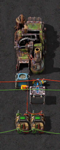
It performs the following steps:
- The inserter will move exactly 1 repair pack into the recycler.
- The recycler will recycle the item, and upon completion query the RNG for 2 new integers, determining whether extra items (either 0 or 1) are produced.
- Depending on whether the items are produced or not, they are placed into the provider chest. This chest is set to read the contents, providing the observation to the red wire.
- These observations directly correspond to the topmost observed bits due to the 50% chance of output. Further processing occurs through the decider combinators below.
- Before the next call can occur, we clear the provider chest by making use of the trash unrequested option, alongside the enable/disable signal we can send over the green wire connected to it, which temporarily pauses the auto trashing behavior when the requestor chest is disabled. Otherwise it requests no items.
The above unit will therefore always provide us with 2 bits of information. To reconstruct the full state quickly, we copy this unit 44 times, yielding a total of 88 bits. This then looks like:
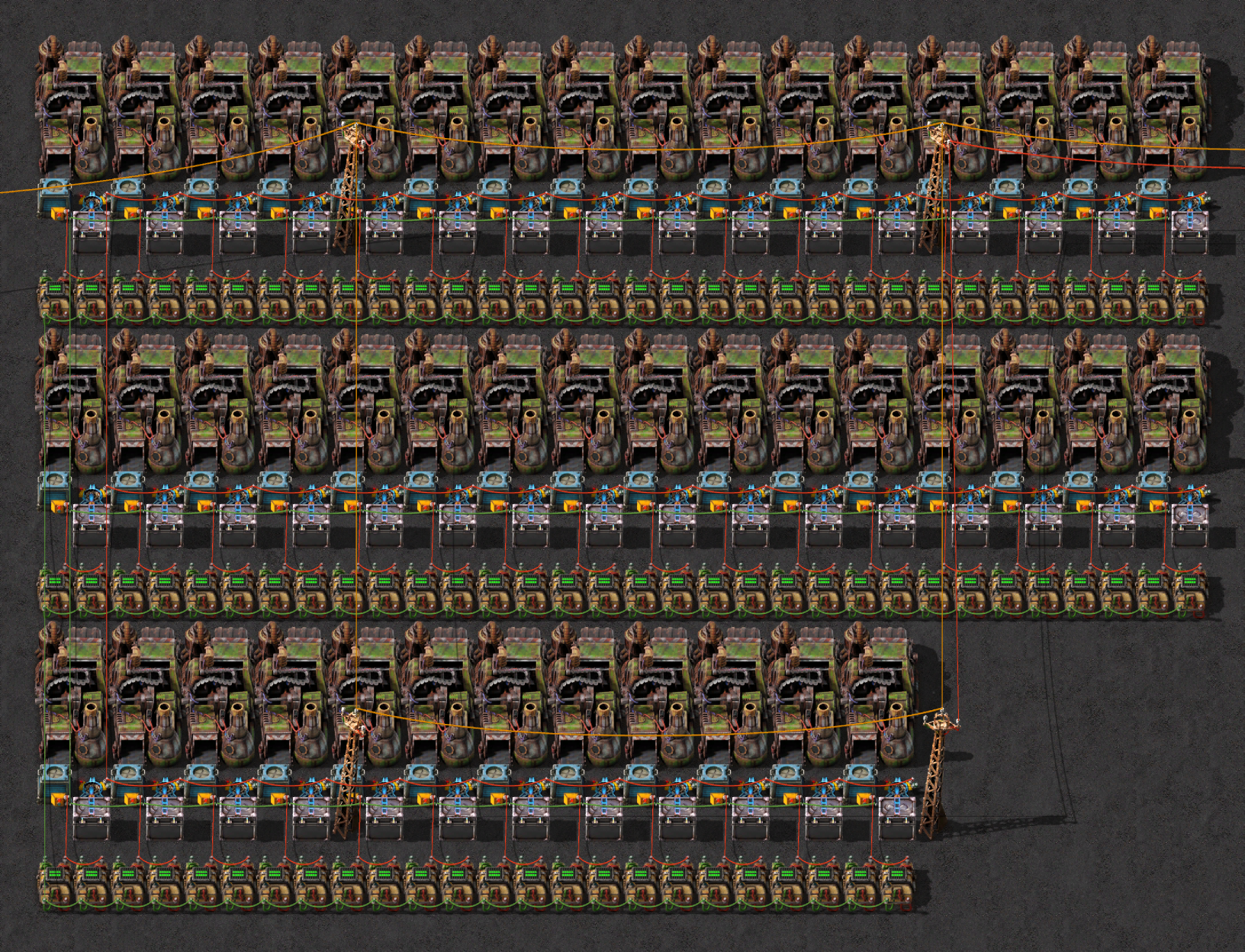
Of note here is the manner in which the individual units are queried. There are 2 approaches:
- Either each is triggered with a 1 tick delay, ensuring that they are always queried in the same order. This, however, requires us to not have any other RNG running in the meantime, as RNG calls which occur in between will mess up the expected ordering.
- Alternatively, we can use same tick shenanigans. By splitting the red wire connecting the inserters with a 1 tick delay combinator in front of every inserter, this can be achieved. Connecting the inputs to the delay first creates a shared circuit network. Then sequentially connecting all outputs of the delays to the corresponding inserters will create a standalone network for each inserter. As the game needs to update the networks in some manner, I bank on the fact that it will iterate through the list ordered by the network ID. This ensures that the RNG calls all happen in the same tick, with no ticks interfering. Note that the wire construction can also be done using a 2-stage blueprint.
While the same tick stuff seems to work in practice, I have not actually confirmed that this is how the game works under the hood. It can be brittle at times, as it seems to arbitrarily break at random times. In those cases, simply reconstructing the wires allows it to work again.
Determining the current state
Each unit produces only single bit observations as a result, so we need to apply a similar strategy as we did before. This time though, we only use the first row of the linear equation defined above for computing observations from the state:
where is the first row of the matrix . If we now let be the matrix which denotes performing RNG steps followed by an observation of the topmost bit, then we can write the observations we gather above to follow the subsequent equation:
Now, as we consume 88 calls when we perform our observation, it would be beneficial to instead directly calculate the state the RNG will be in after our observation, rather than when we started. This can be achieved by making use of the inverse transition matrix which causes some shift in the time index, creating a new matrix :
Shifting the time to be relative to the next RNG call by means of substituting we then arrive at the equation:
This can be read as us computing the next internal RNG state from the previously done observations. Now since there are only 88 bits which are actually linearly independent, we cannot compute a full inverse. However, a pseudo-inverse will suffice. Especially since we are interested in the states after – for which the lowest bits are entirely described by the most significant bits. This means that even a single step forward will deterministically set those previously unknown bits, so we are all fine.
The really neat thing about this entire endeavor is that matrix and similarly do not depend on any dynamic state. As such, can be precomputed in Python and subsequently used in Factorio.
Hence we only need to implement a matrix-vector multiply in in-game. To do so, remember that any matrix-vector product can be seen as a weighted sum of the matrix columns weighted by the entries in the vector:
In this case, as we are performing our computations in , each entry is either 0 or 1, meaning the multiply can be represented with a simple conditional, while the sum is substituted with an XOR over all the weighted vectors:
Here is the -th column of while is the -th bit observation performed. In practice this equation is computed in 2 parts.
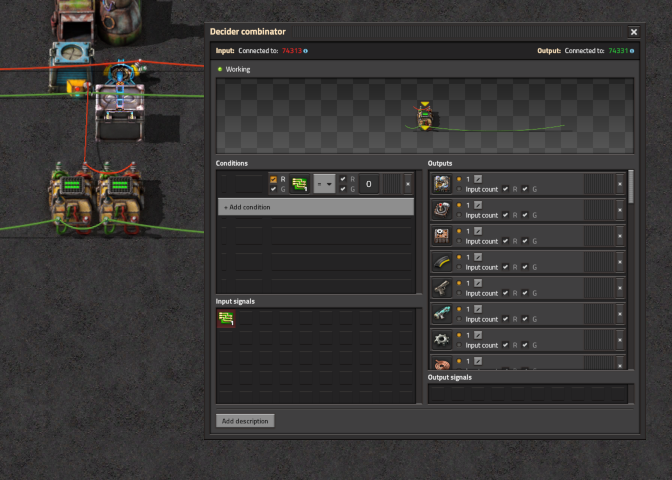
First, each measurement unit computes a pointwise scalar-vector multiplication of and vector . This is done via the decider combinator mentioned above doing “further processing”. If the resulting item was not observed () then the roll was above the threshold and we have , meaning this column needs to be accumulated otherwise it is not. The vector is stored in the constant outputs of the decider combinator, where only the bits which are 1 are actually output. As such the vectors are represented by 96 different signals.
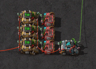
Finally we require the XOR of all these vectors to obtain the final state. This can be achieved via implicit addition.5 Summing the values of a single signal and extracting only the last bit of this sum is equivalent to taking the XOR over all of them. As such, by wiring all decider outputs together, a single arithmetic combinator can perform the bit extraction by ANDing the pointwise sums with 1.
As each signal now corresponds to a single bit of the 3 32-bit LFSR states, we can make use of a set of decider combinators to sum up all the corresponding bits of each active signal. Thus we have 3 signals, each containing the current state of the game’s RNG.
Looking into the future
We perform a similar action to compute the future states of the individual LFSRs. However, as all LFSR states require fewer than 32 bits, we can store the lookup table in a more compact fashion. For each LFSR we need to compute the following:
This is computed for , where and are different between the 3 sub LFSRs. From this we can again rewrite these matrix-vector multiplications as:
where is the -th column of . These columns can be stored as 32 bit integers, as . Hence the skip-ahead equation can be implemented in parallel for all steps as follows:
- Split the packed state into its individual bits . Represent these as individual signals again (arithmetic combinator on the left).
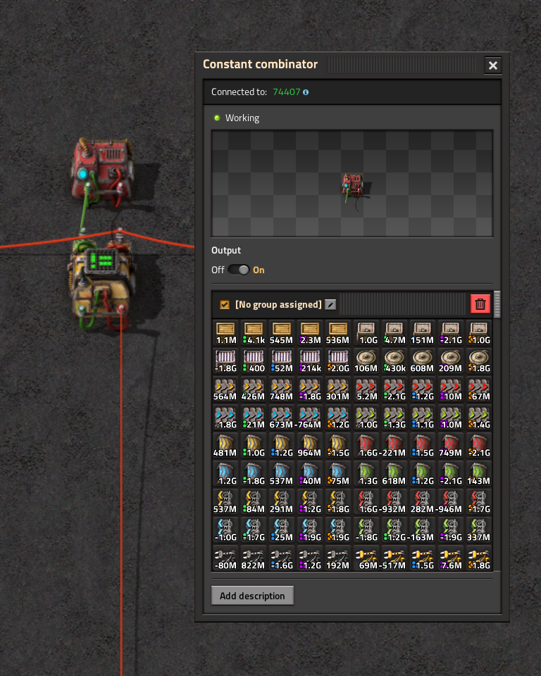
- The pointwise scalar vector multiplication with all the different vectors will either include all the vectors in the corresponding -th state or not, thus we can implement this via a decider combinator again. This time, however, I store the constants in a separate constant combinator – it can output more signals at once. I opted to predict 1000 forward steps in parallel.
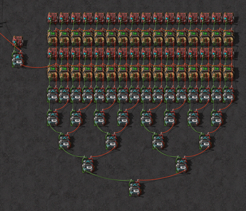
- Now we have 32 nets each full with 32 bit wide values which need to be XORed together. Unlike before we cannot utilize the implicit addition here, as the vectors are now not represented by 32 different signals but instead via a single 32 bit signal value. Thus we have to use more arithmetic combinators. I’ve opted to use a binary tree to pairwise XOR sets of vectors together, as this is a known fast reduction strategy for prefix sums (which this is).
Quality prediction
Now that we have the next RNG call results before the actual in-game calls
happen, we need to make them usable for our purpose. This basically means implementing
some form of the rollQuality function from the game.
A reverse-engineered version of the function can be seen below, implemented in pseudo-C++:
// Fixedpoint value of the module effect from -32.768 to 32.767
// e.g. 10% quality would be a value of 100
typedef EffectValue int16_t;

// Stub of relevant quality prototype fields
struct QualityPrototype {
    ID<QualityPrototype, uint8_t> id;
    ID<QualityPrototype, uint8_t> next;
    double nextProbability;
}

// Mapping from the ID<...> to QualityPrototype
PrototypeList<QualityPrototype>::indexToPrototype;

// Function which determines crafting result quality
ID<QualityPrototype, uint8_t>* QualityPrototype::rollQuality(
  ID<QualityPrototype, uint8_t> qualityID,
  EffectValue bonus,
  RandomGenerator* generator,
  IDIndexedData<uint8_t, ID<QualityPrototype, uint8_t>>
    const* unlockedQualities
) {
  // If no bonus, do early return -> no RNG call!
  if (bonus == 0)
    return qualityID.copy();

  QualityPrototype* quality = indexToPrototype[qualityID];

  // Roll the RNG exactly once
  double roll = RandomGenerator::uniformDouble(generator);

  // If roll < threshold we upgrade to the next quality
  double threshold = (double)((float)(bonus) / 100f);

  // Find highest quality which beats the threshold
  uint8_t nextIndex;
  while ((nextIndex = quality->next.id.index) != 0) {
    if (!unlockedQualities->data[nextIndex])
      break;

    // Scale by next upgrade probability, base game = 0.1
    threshold *= quality->nextProbability;
    if (roll > threshold)
      break;

    quality = indexToPrototype[nextIndex];
  }
  return quality->id.copy();
}
If we take a look at how the function is implemented in the game we can see that it basically just takes the RNG roll and compares it against some thresholds. It stops as soon as it finds a threshold which is no longer beaten by the roll.
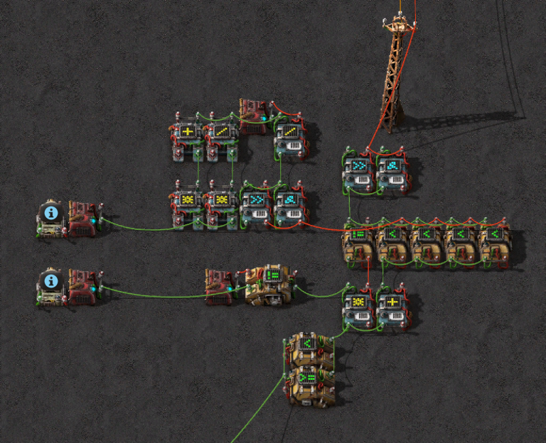
This means that each craft which involves quality rolls will take exactly 1 RNG call. And for each call we can compute the expected quality level by just comparing against all the thresholds, which stay constant during the game. Thus they can be precomputed in-game with some arithmetic combinators.
The calculator below shows the required threshold for each quality level, as well
as the expected amount of each quality level for a given bonus.
Note that when the threshold exceeds , i.e. the uint32_t maximum value,
we always upgrade, which is indicated by placing the thresholds in brackets.
| Result | Probability | uint32_t Threshold |
|---|---|---|
| 75.200% | 1,065,151,889 | |
| 22.320% | 106,515,188 | |
| 2.232% | 10,651,518 | |
| 0.223% | 1,065,151 | |
| 0.025% | 106,515 |
Adapters
Yippee, we can now compute the relevant RNG outcomes before the corresponding calls even occur in-game. Now the question is what can we do with that? I have by now experimented with several – what I call – adapters, which take in these predictions, and do some funny stuff with them.
Beginning with the first that I’ve implemented:
It takes the sequence of future output qualities, and displays them next to the assembler, similar to the “Next Up Pieces” queue in Tetris. Each time a craft is completed, it advances the window into the future outputs by one, keeping the display relevant at all times.
The next one was the following:
This one takes the same list, but instead assigns only a single crafter to fabricate the next item. The assembler which is selected depends on the next output quality. In turn this leads to the 5 assemblers outputting the items in a sorted fashion, where each belt only ever carries a single type of quality, ordered from left to right in increasing quality.
Finally, the goal that I’ve been interested in from the get-go – and the hook already seen at the start of this post:
This method encapsulates the entire prediction and crafting loop into a closed system, which can do the entire thing (predict and craft) autonomously. We have seen how we can compute the current state, and predict the next states. But how does this let us force RNG values of our desire?
The answer is the simplest of all: It doesn’t. At least not directly.
Instead, we can make use of the fact that the sequence of the RNG outputs is deterministic. By consuming the bad RNG calls which would need to occur before our desired one, we can “force” the RNG to next output a desired value – such as one which upon use in the quality rolling code immediately upgrades from common to legendary quality. For this we need something to consume the RNG calls.
One automatable aspect is again the creation of partial item stacks. Unlike before however, we do not care about observing the output of these crafts, but only the number of calls each crafting cycle makes. Additionally quick crafting cycles lead us to maximize the number of calls per second.
As luck would have it we already saw a recipe which consumes many calls and has a tremendously fast crafting speed: Scrap Recycling. It takes 12 calls per completed craft, with a base speed of 0.2 seconds. Note that this holds for the number of completed crafts, i.e. crafts completed by productivity count as well. While this for one means that we scale the calls consumption rate of each recycler with the infinite scrap recycling productivity, this simultaneously also requires additional handling of the productivity.
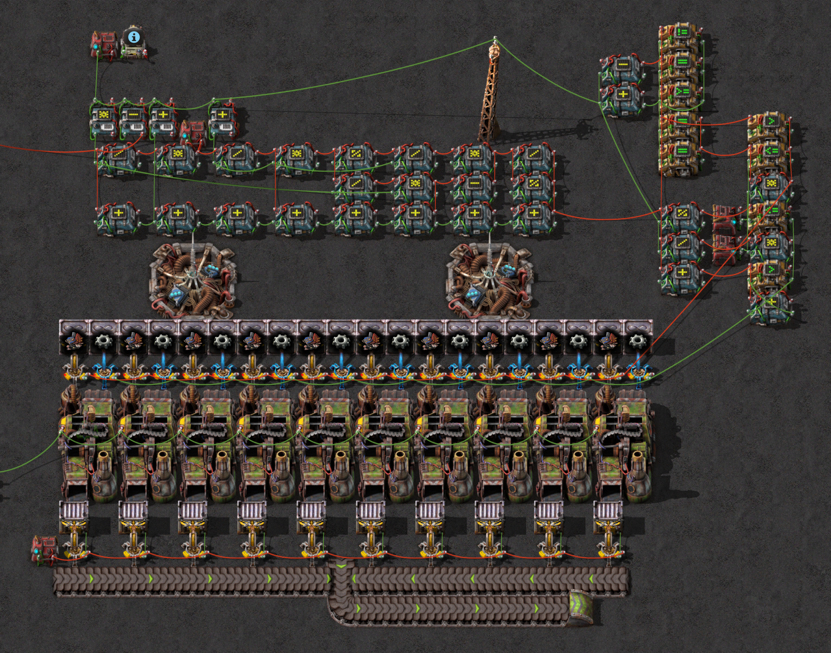
Using scrap adds complexity due to the following considerations:
- We have multiple recyclers, so we need to figure out how much scrap each gets, and how many get an additional one? The last part helps reduce the number of items of the last stage.
- Recycling scrap steps rng calls per craft which is not fine grained enough to resolve an exact state. The remaining number of necessary calls are padded with crafts only eating a single call each. Here these are gears.
- We also need to consider crafts completed due to scrap recycling productivity which occasionally leads to multiple crafts finishing for a single input item. This causes the RNG to be queried for multiple recipe results, i.e. a multiple of the 12 calls.
- Each recycler is started with at least 1 gear before scrap to reset the previous productivity progress allowing us to avoid tracking that as well.
The exact function implemented
To implement the exact function I first wrote some code to simulate it, then let AI derive a closed formula which I could simplify and translate to combinators. The relevant notebook can be found here. In short: we require a function which computes given recyclers and productivity level for any desired number of calls , how many scrap each recycler gets where many get an additional one while is the number of additional gears consumed.
The equations can be written as:
where are craft completions, the step size if one more craft completes, the number of recyclers, and the number of RNG calls.
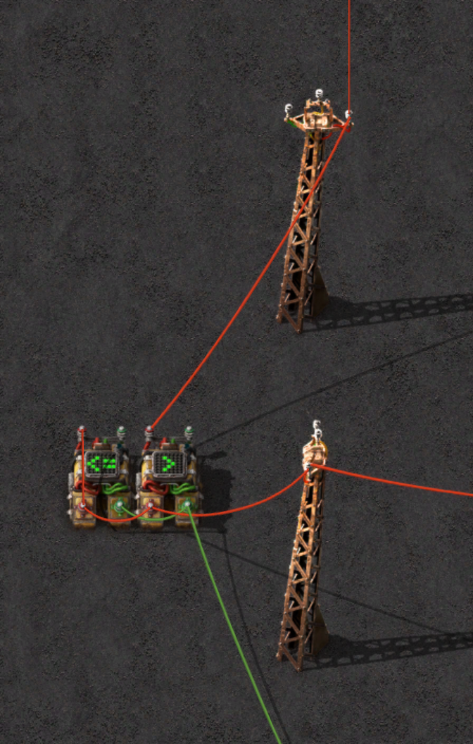
There are two additional considerations to make. First of all, while we could increase the amount of calls simultaneously predicted in the forwards pass, this will bloat the save / blueprint and does not scale well past a couple thousand calls per pass. Instead, we can simply feed the output of the last computed RNG states back into the RNG forwarder in a feedback loop.
The first 2 adapters could simply ingest the output of the quality prediction module. To somewhat decouple the prediction and skipping ahead, I decided to decouple the 2 systems, by buffering known good offsets.
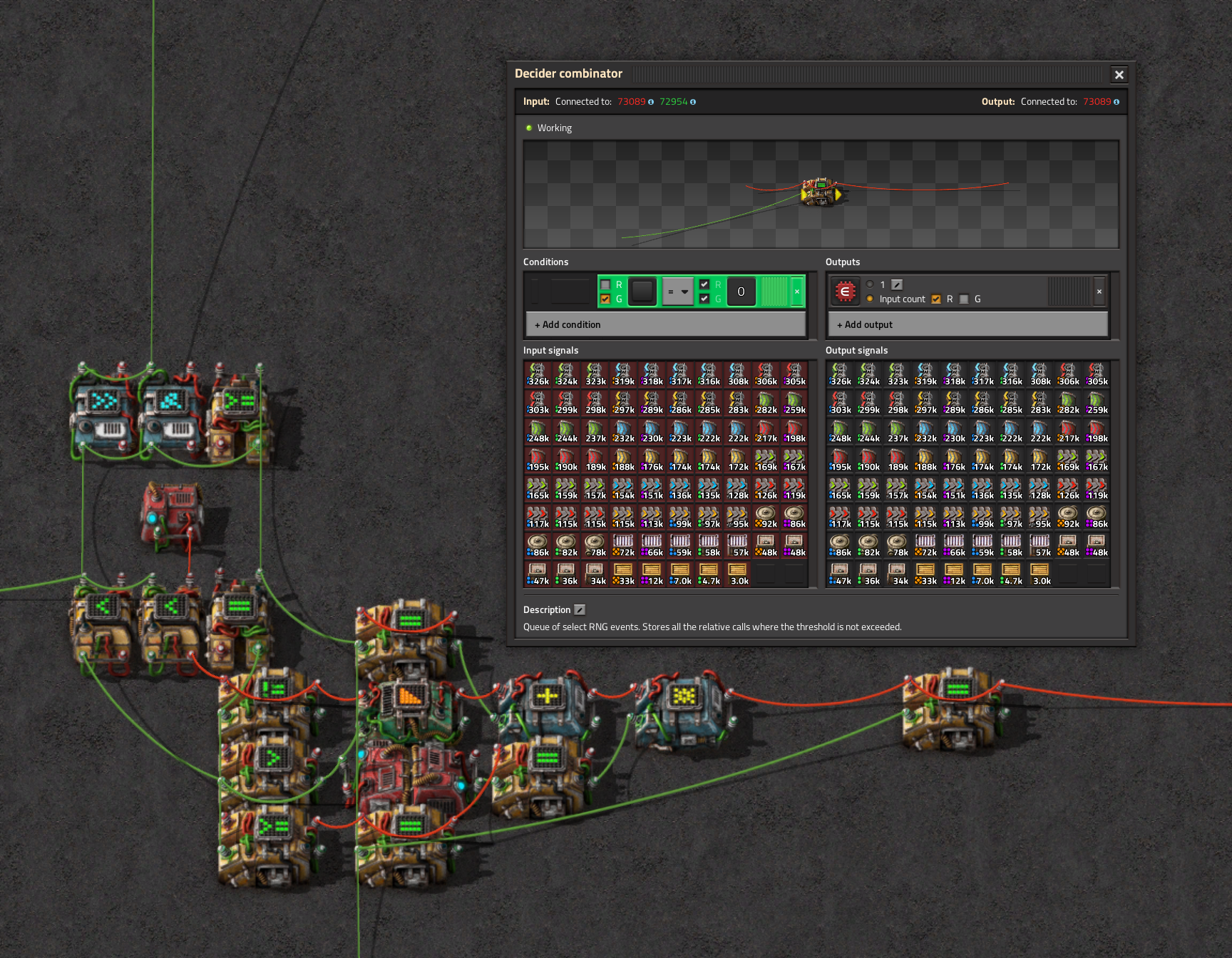
For this, as before I compute the threshold which needs to be passed, and now unlike before: Filter out the relevant call indices / offsets and only store those instead. This is done by remapping the passing signals into a sequence of new signals, one for each good offset, as seen in the image below. The remapping is done at 1 signal per tick. Once all passing signals of this iteration are consumed, the above feedback loop is triggered to advance to the next 1000 steps.
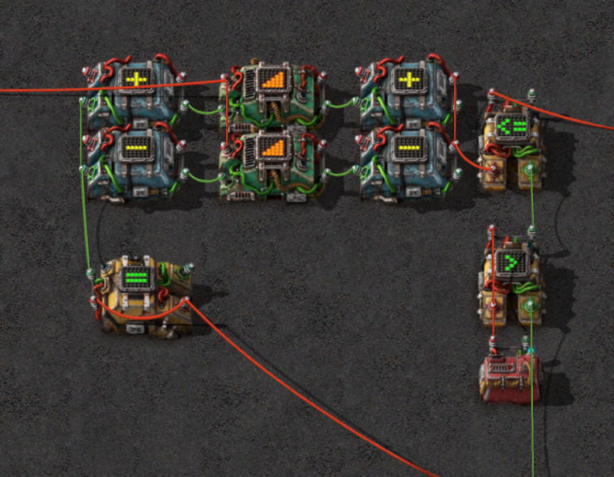
As this buffer stores absolute offsets from the first time we measured the RNG, we need to compute the number of calls to actually skip to arrive at the next index. For this we fetch the current and the next index from the buffer and subtract their offsets, yielding the delta. This delta is then what is actually fed towards the skipper. The next number of steps is fetched only after the skipper has finished with the current cycle of skipping and creating the next item.
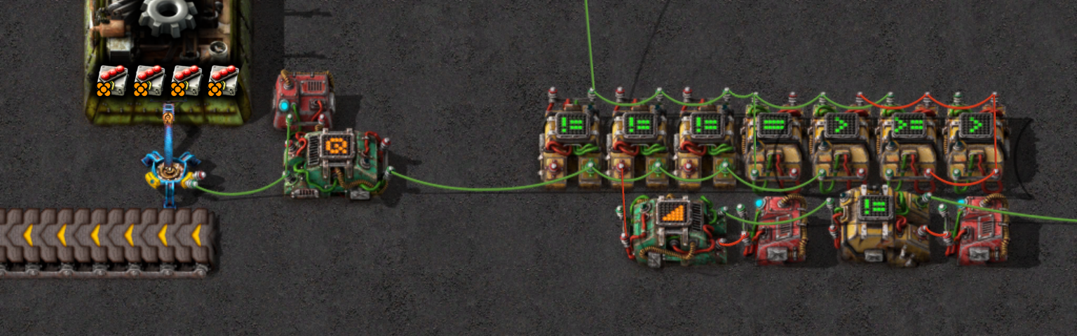
Lastly, we have the issue that the simulated registers may diverge from the actual game RNG state – for instance if any other process has consumed a RNG call unbeknownst to us. While we can not prevent such intermittent calls, we can at least detect them. In this instance our predictions will diverge from the actually observable crafting results. As such, when too many results (2) differed from our expected quality, we can simply restart the machine automatically, triggering another full state observation and forwarding future states from there on.
Below we now see the entire machine in its full glory. I’ve highlighted the different modules corresponding to the individual segments we constructed previously. The general data flow can be read as starting from the bottom left (the assembler) going clockwise: Readout (lime), prediction (blue), filtering (yellow), buffering (purple), skipping (black).
Limitations
Now to the important part, that you may be wondering about:
Sweet! Can I use this to now do <insert RNG manipulation target> in my save-game?
The short answer: Very unlikely.
But why? It’s not that I want to keep this tech for my self. In fact, here is the world download, a blueprint string and the relevant cleaned up python code for you to play with. No, it rather has to do with the way that Factorio currently handles their random generators.
For this we can take another look into the game binary.
After browsing a bit we encounter the Map object, which among other things as references to the individual surfaces (i.e. the different layers of the world, like the planets Nauvis, Fulgora, and so on).
The RNG states however are not stored per surface, but rather globally for the entire map.
And notice that I am speaking of states (i.e. plural) as there are actually multiple RNGs in game,
each responsible for some of the game’s logic.
The Map in particular stores the following six RNGs (names from the pdb).
Try to guess what each one is responsible for:
Map.aiRandomGeneratorMap.entitiesRandomGeneratorMap.generalRandomGeneratorMap.mapRandomGeneratorMap.triggerRandomGeneratorMap.unsafeRandom
To be honest, I still don’t know what some of them do, I was only interested in the one relevant to item crafting procedures.
Additional RNGs
There are more generators in the binary, the full list I have currently found in addition to the ones mentioned above is:
GlobalContext.randomGeneratorLightningMeshGenerator.randomSelectorCombinatorControlBehavior.randomSoundRandomizer.randomGeneratorSpacePlatform.asteroidsRandomGenerator
To try and track all the RNGs and what potential call paths are which lead to a random number call,
I made use of binary ninja and its python scripting to extract a call tree originating from the RandomNumberGenerator::getInt call and its derivatives.
The corresponding scripts for scraping are available here.
Here we can already see a saving grace for RNG manipulation. Not all random effects are handled by the same RNG, and thus we can at least isolate some of them from the rest of the game logic. For instance, the RNG responsible for the biter spawning and pathing is separate from the RNG we are interested in.
In particular this is the generalRandomGenerator, which is responsible for the item creation.
As its name implies, it is the general random generator, meaning there is still some overlap with other game logic.
Either completely unrelated to item creation, or through other recipes which also have probabilistic outputs.
This is exactly the issue with the non-isolated cases I talked about previously.
First a non-exhaustive list, of instances unrelated to quality rolling:
- Floor tiles changing via the
MapGenerator::clearEntitiesAndSetTilefunction, which randomly chooses from variants. This can happen due to manual edits via the editor, through the freezing logic changing tiles, tile ghosts being constructed, or a space platform building some flooring. - Name randomization of entities like labs and train stops,
- Player manually mining ore (particle spawning) or walking over dusty ground (creating dust particles),
- Particles in general i.e.
ParticlePrototype::getRandomVariationandSmokeconstructor, - Selector combinators initialize their own RNG with a random seed,
- Mining drills with a single ore tile running out randomly shuffle all remaining tiles they mine,
- Lightning strikes on Fulgora,
- Spidertron leg placements when walking
Secondly, all machines requiring any sort of randomness share the same RNG. Any time another (by my machine unexpected) recipe uses the RNG – for instance your scrap recycling line on Fulgora, uranium processing on Nauvis, or any other quality rolling – then the state of the RNG will change, causing the predictions of my machine to diverge from the actual game state, making it impossible to reliably manipulate the RNG towards any specific goal. Moreover, consider that in a game about automation one usually scales up to produce large volumes of items, leading to potentially thousands of calls occurring in just a second, outpacing my capabilities of precomputing the RNG fast enough.
While it might be possible to account for all / many of the randomness sources above, e.g. by dynamically disabling any other production lines doing random calling using for example a logistics group, and waiting for daytime on Fulgora it may be possible to apply this in an actual game save, it should be taken into account from the get-go, rather than being retrofitted into an existing save.
Factorio 2.1
With the last major update to Factorio, the way the RNG is used has changed.
While they still use taus88 as the underlying generator, they have fundamentally rewritten major parts of the item creation logic, reusing a single call for multiple item outputs.
Additionally from what I can currently tell, now every single crafting operation uses the RNG, even if it is deterministic, to fill the shared call field in case anything later on will require it. This means that no other machine can run in parallel, as it will always interfere with the RNG state.
Moreover, due to the sharing of the rolls, using scrap recycling to skip the RNG forwards is no longer useful, as the RNG is queried the same amount for any recycled item, and dealing with scrap recycling productivity and its many outputs increases the overhead a bunch. As such this could be replaced with the recycling of any other simpler/cheaper item instead – at least it’s no longer directly bound to Fulgora.
Lastly, while the update is still in the experimental branches I have been somewhat on a rollercoaster ride seeing different changes to the RNG system.
At one point, the Map::generalRandomGenerator was used to control the FISH motion.
This of course would be a huge problem, as it meant that any fish on the map generated an unknown number of RNG calls, leading to it continuously desynchronizing the RNG state from the predictions without any feasible way to account for it shy of removing all fish from the map (without generating any new chunks with new fish).
Thankfully, this was changed in a later update (its gone in version 2.1.13) with a new seventh RNG on the Map object, called Map::fishRandomGenerator. Guess what its job is :)
However its not all bad. For instance, with the forced move away from scrap recycling, and the addition of universe wide signals (allowing us to send when Fulgora lightning storms start to other planets) we are no longer bound to any specific planet, and could instead build the manipulator on Vulcanus, gobbling up however many resources the skipping now requires, sending a signal to any other planet to craft local legendaries when the RNG is in the right state.
For now, I will leave it at that, as the game may further change while it is still in experimental, so any updates to the cracker might just get broken by the next update without notice.
Conclusion
This marks the completion of a two+ year project, finally reaching the fully autonomous gamblen’t I wanted from the beginning. Though to be fair, most of the latter part was me procrastinating on writing and publishing this post. In the meantime (while I was dragging my feet), others have also looked into the RNG, who I’ll link here for reference:
@kovaxisin the Factorio forums, reaching and stopping at a similar point as I did initially, where the state is computed with an external python script from some in-game observations.@d4s_over_dt4on the Factorio discord, who built a combinator circuit to compute the RNG state, read out from 3 placed selector combinators (which each query the general RNG to seed each combinators own state), without further followup integration or verification.
Boy there were quite some tangents along the way which did not even make it into this post, as its long enough already, such as me partially recreating cnide with improved handling for subnets just for documentation and simulation purposes as with syntax highlighting in vscode, or the first implementation attempt where I did all the matrix math in game, including the creation of the matrix and Gaussian elimination of said matrix.6
Thanks go out towards
@earthcomputerand co. who unknowingly inspired this project, as their “Mess Detector” reads out Minecrafts RNG state with only in-game mechanics,@redruin1with their factorio-draftsman library allowing for easy procedural blueprint creation,- the Binary Ninja team for a decompiler which
does not shit itself7 actually works when encountering the relatively chonky factorio.exe, - and everyone close to me who bullied me into finally finishing this writeup after hearing me rambling about RNGs for the past 2 years :)
- See Factorio Friday Facts #375↩
- Trivially breakable for security researchers seems to mean that they know how to break them, hence its easy, even if still takes some setup to understand.↩
- This part of the project is where I realized that structures like Field, Ring, Monoid are basically the mathematical variant of programming using generics, where we can write algorithms which work for any type which satisfies the necessary properties. And just like when programming anything, the naming often sucks :) But somehow sticks… ↩
- Factorio actually provides a way to dump the data by running with command line arguments.
One of these is
--dump-datawhich outputs a JSON file containing the processed prototypes as they are loaded in-game. This can then be parsed for further processing, such as extracting the various recipes. However, I just used the data bundled with draftsman.↩ - In Factorio, when multiple devices write a signal to the wire, then the resulting signal value on the wire is the sum of all the individual signals. This means any summation can be done implicitly.↩
- The Gaussian elimination in game is actually also included in the world download, with some instructions on how to use it.↩
- Unlike ghidra, where even 64 GB RAM were not enough to successfully decompile the game exe.↩